Flux Data Processing – Workflow Summary
Utah Geological Survey – Flux Monitoring Network
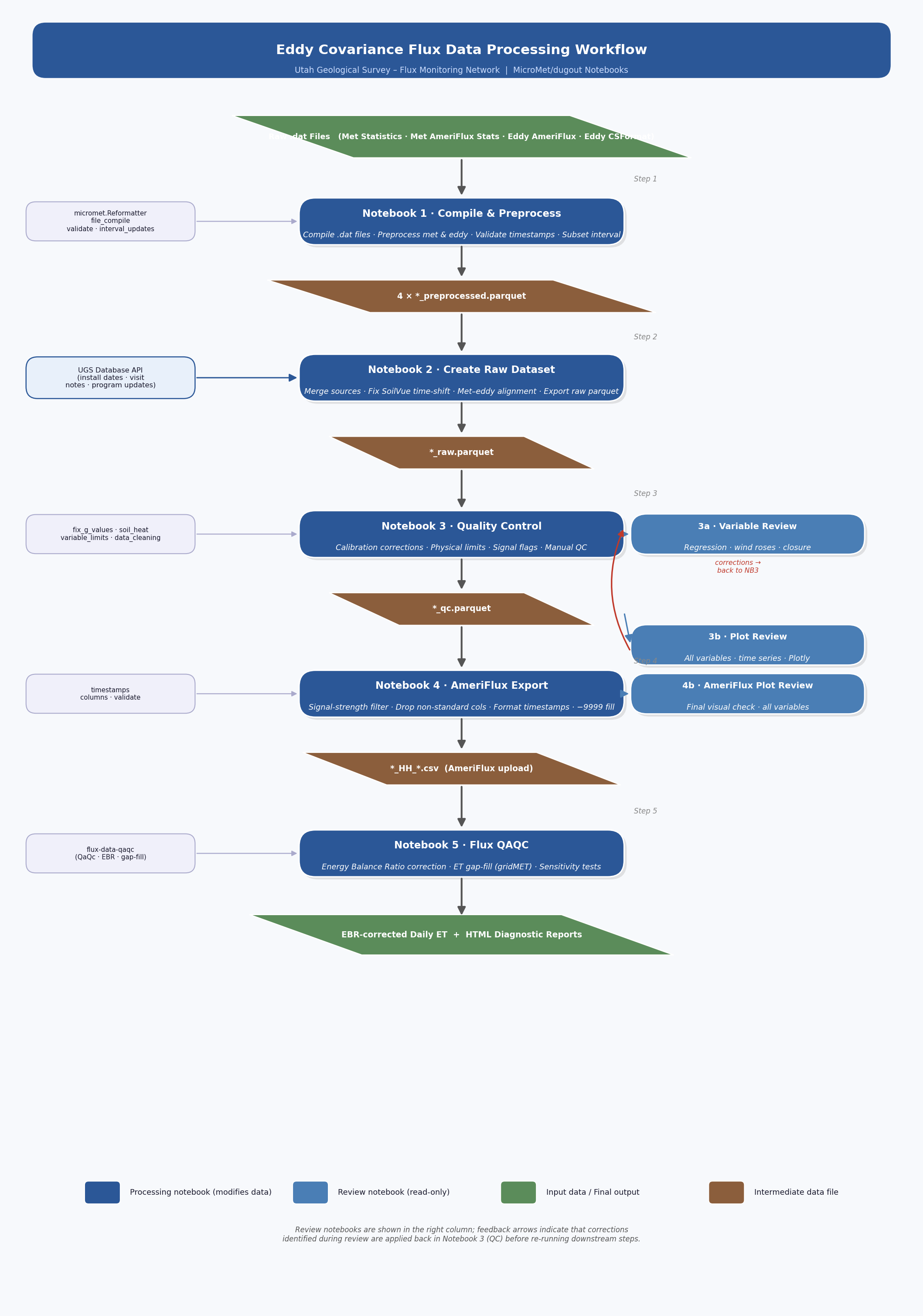
This page provides a high-level overview of the eddy covariance data processing pipeline. For full technical detail on each step, see the complete workflow reference.
Workflow Flowchart
Pipeline at a Glance
The pipeline converts preprocessed eddy covariance and meteorological data into quality-controlled, AmeriFlux-formatted output through five processing steps and three review checkpoints.
Step |
Notebook |
Input |
Key Operations |
Output |
|---|---|---|---|---|
|
Raw data logger or EasyFlux web files |
Compile datalogger files · standardize columns |
|
|
|
Preprocessed parquets |
Merge data from different data streams · Merge met and eddy data · fix time alignment issues |
|
|
|
|
Calibration corrections · physical limits · SoilVue G calc · manual QC · signal flags |
|
|
|
|
Signal-strength filter · drop non-AmeriFlux columns · format timestamps |
|
|
|
|
Gap-fill redundant sensors · EBR correction · ET gap-fill · sensitivity tests |
Daily ET + HTML reports |
Review notebooks (read-only – findings feed corrections back into Step 3):
Notebook |
When to run |
Purpose |
|---|---|---|
After Step 3 |
Summary statistics, distributions, outlier detection |
|
After Step 3 |
Quick time-series sweep of every variable |
|
After Step 4 |
Final visual check before AmeriFlux submission |
Step-by-Step Summary
Step 1 – Compile & Preprocess
Create compiled and clean versions of data from each data stream (e.g., CSFlux web/datalogger, AmeriFlux eddy web/datalogger, MetStats, MetAF)
Organize datalogger files into a single directory by table name (e.g., Statistics_Ameriflux, Statistics, Flux_AmerifluxFormat, Flux_CSFormat)
Compile data from a single data stream into a dataframe
Clean data by applying renaming dictionary, setting data types, and fixing timestamp issue
Subset out data to only include 30 or 60 minute data, depending on user input
Present data for review to identify misnamed columns and missing data
Export data into separate parquet files for data from each data stream
Output: {station}_{timestart}_{timeend}_preprocessed.parquet
Step 2 – Create Raw Dataset
Assemble multiple preprocessed files into final datasets and manage any datetime shifts
Load preprocessed parquets for each data stream (CSFlux web/datalogger, AmeriFlux eddy web/datalogger, MetStats, MetAF)
Compare and merge eddy data – CSFlux and AmeriFlux eddy streams are compared for differences; the AmeriFlux stream is primary, with CSFlux filling gaps and providing unique columns (e.g., G_PLATE, diagnostic fields)
Compare and merge met data – MetStats and MetAF streams are compared and combined
Detect and correct temporal shifts – SoilVue sensor data (EC_3_, K_3_, SWC_3_, TS_3_) may be offset by one time step; cross-correlation detects the lag and a frequency shift corrects it. Historical timestamp misalignments are also identified and corrected.
Combine eddy and met – merge the two streams, resolve duplicate columns, validate 30-minute interval integrity
Standardize column naming – apply AmeriFlux positional suffixes (_1_1_1, _1_1_2, etc.)
Trim to station record – drop data before the station install date (retrieved from the database API)
Output: {station}_{timestart}_{timeend}_raw.parquet
Step 3 – Quality Control
The largest and most site-specific step:
Calibration corrections – date-gated fixes for soil heat flux storage thickness, precipitation calibration factors, and G_PLATE sign inversions
SoilVue G calculation – derive ground heat flux from temperature/moisture profiles using the
soil_heatlibrary (Johansen thermal model)Physical limits –
Reformatter.finalize()applies range limits, converts SWC units, standardizes SSITC encoding, and produces a limit reportManual corrections – field-day precipitation, G_PLATE zeros, SoilVue spikes, wind direction offsets, sensor-specific spike removal
Signal-strength flags – H2O/CO2 signal flags (0/1/2) and wind direction obstruction flags
Gap-fill G – linear regression between redundant G sources to impute missing values
Output: {station}_{daterange}_qc.parquet + limit report CSV
Review: 3a & 3b
Run after Step 3 to evaluate data quality. Issues found here are resolved by adding correction blocks in Notebook 3 and re-running Steps 3–5.
3a: Summary statistics, data availability, and outlier detection for each variable.
3b: Interactive Plotly time-series for every column – a rapid visual sweep for spikes, gaps, or artifacts.
Step 4 – AmeriFlux Export
Converts the QC dataset into an AmeriFlux-compliant half-hourly CSV:
IRGA-derived variables set to NaN where signal strength < 0.8
Non-AmeriFlux columns dropped; all-NaN columns removed
NaN replaced with -9999; timestamps formatted as
YYYYMMDDHHmm
Output: {station}_HH_{start}_{end}.csv
Step 5 – Flux QAQC
Runs fluxdataqaqc for energy balance ratio (EBR) correction and ET gap-filling:
Gap-fill redundant NETRAD and G sensors via linear regression
EBR correction applied to LE; ET gap-filled using ETrF x gridMET ETr
Data subset by year and season for analysis
Sensitivity runs with different Rn/G input combinations
Outputs: EBR-corrected daily ET, HTML diagnostic reports, optional daily CSV
Key Libraries
Library |
Role |
|---|---|
Core pipeline: |
|
soil_heat |
SoilVue-derived ground heat flux (Johansen model) |
fluxdataqaqc |
EBR correction, ET gap-fill ( |
pandas / numpy |
Data wrangling and array operations |
scipy |
Cross-correlation and linear regression |
plotly / bokeh |
Interactive diagnostics and HTML reports |
Directory Structure
M:/Shared drives/UGS_Flux/
├── Data_Downloads/compiled/
│   ├── preprocessed_site_data/   ← preprocessed parquets
│   └── {stationid}/              ← raw .dat source files
└── Data_Processing/final_database_tables/
    ├── raw/          *_raw.parquet
    ├── qc/           *_qc.parquet
    └── ameriflux/    *_HH_*.csv
Adapting to Other Sites
Copy the notebooks and update:
station,interval,date_range– station code, measurement interval, and date boundsCalibration correction dates and factors (Notebook 3)
Sensor failure date ranges and affected variables
Wind direction offsets between instruments
Signal-strength bad-period date ranges
Column selection for eddy merging (Notebooks 1/2) and AmeriFlux export (Notebook 4)
.iniconfig forfluxdataqaqc(Notebook 5)
See the full workflow document for detailed guidance.